NMR Spectroscopy of Proteins Explained for Researchers

Q: What is NMR spectroscopy of proteins in simple terms?

NMR spectroscopy of proteins uses strong magnetic fields and radiofrequency pulses to detect signals from atomic nuclei in a protein, revealing its 3D structure, how it moves, and how it interacts with other molecules, all without destroying the sample.

Q: Why is protein NMR considered difficult?

The main challenge is protein flexibility: proteins sample multiple conformations across many timescales, so NMR data reflects a dynamic ensemble rather than a single structure, requiring careful integration of spatial and temporal information to interpret correctly.

Q: How much protein do you need for an NMR experiment?

Typical NMR experiments require approximately 2–30 mg of isotopically labeled protein in 260–550 µL of buffer, with roughly 10 mg being a practical target for an 8–30 kDa protein at 0.5 mM concentration.

Q: What is the main purpose of NMR spectroscopy for proteins?

NMR provides atomic-resolution information about protein structure, dynamics across timescales from picoseconds to seconds, and molecular interactions, including weak and transient binding events that are invisible to most other structural techniques.

Q: Can NMR detect binding events that other methods miss?

Yes. NMR detects millimolar-affinity ligands through chemical shift perturbation and can reveal low-population excited states populated at as little as ~1%, making it the method of choice for fragment screening and allosteric site identification in drug discovery.

TL;DR:

NMR spectroscopy of proteins is a non-destructive technique that reveals site-specific structure, dynamics, and interactions. It is unique in capturing motion and detecting weak or transient binding events, especially beneficial for studying intrinsically disordered regions and drug interactions. Although demanding in sample preparation and instrumentation, NMR provides insights that are often unattainable by other methods.

NMR spectroscopy of proteins is a non-destructive, atomic-resolution technique that reports site-specific structure, dynamics, and molecular interactions in solution, solid state, and living cells. Unlike X-ray crystallography, it does not require a crystal, and unlike cryo-EM, it captures motion. When your question is how a protein moves, where a ligand binds even weakly, or what an intrinsically disordered region actually does, NMR is often the only method that gives you a direct answer.

The practical constraints are real: routine protein structure NMR works best for proteins in the 5–25 kDa range, samples typically need to be at sufficient concentration, and full structure determination takes weeks to months of instrument time and analysis. For larger systems, specialized methods (TROSY, perdeuteration, methyl labeling) extend the range but raise the complexity.

Quick reference before you read further:

Structure: NMR determines 3D protein structure in solution from distance and angle restraints.
Dynamics: It probes motion from picoseconds to seconds, including low-population excited states down to ~1% occupancy.
Interactions: Chemical shift perturbation maps binding sites and quantifies affinity for weak ligands.
Sample: Plan for 0.1–1 mM protein, 260–550 µL, isotopically labeled (¹⁵N, ¹³C) for most experiments; approximately 10 mg of labeled protein is typical for an 8–30 kDa protein at 0.5 mM concentration.
First experiment: A 1H-¹⁵N HSQC is the standard fingerprint; run it before committing to a full campaign.

What is NMR spectroscopy for proteins, and how does it work?
What can NMR actually tell you about a protein?
Which experiments do you actually run for a protein?
Why isotope labeling is non-negotiable for protein NMR
How to prepare a protein sample for NMR
What instruments and hardware do you need?
What are the real strengths and limitations of protein NMR?
From FID to structure: software and data analysis
How NMR supports drug discovery and fragment screening
How long does a protein NMR campaign take, and what does it cost?
How NMR data integrates with computational workflows
Key Takeaways
NMR's unique value, from where I sit
Innovabiotech's computational services for NMR-driven projects
Recommended further reading and authoritative resources
FAQ

What is NMR spectroscopy for proteins, and how does it work?

Every atomic nucleus with an odd mass number carries a magnetic moment — a tiny bar magnet at the quantum level. Place a protein sample in a strong external magnetic field (B₀), and those nuclei align with or against it, splitting into distinct energy states. A precisely tuned radiofrequency (RF) pulse tips the magnetization away from equilibrium. As the nuclei relax back, they emit a weak oscillating signal: the free induction decay, or FID.

That FID is a time-domain mixture of every resonating nucleus in the sample. A Fourier transform converts it into a frequency-domain spectrum, where each peak sits at a position called its chemical shift, measured in parts per million (ppm). The chemical shift is exquisitely sensitive to local electron density, hydrogen bonding, ring-current effects, and backbone conformation. A glycine in a helix resonates at a different frequency than the same glycine in a disordered loop. That sensitivity is what makes NMR a structural tool.

Three additional interactions shape protein NMR spectra. Scalar (J) coupling arises through bonding electrons and connects nuclei two or three bonds apart, producing peak splitting that reveals connectivity. Dipolar coupling operates through space and is the basis for the nuclear Overhauser effect (NOE), the primary source of distance restraints in structure determination. Relaxation (T₁ longitudinal, T₂ transverse) describes how fast magnetization returns to equilibrium; T₂ shortens as molecular tumbling slows, which is why large proteins produce broad, overlapping lines.

"The significance of NMR progress is evidenced in part by a number of Nobel prizes awarded to its pioneers — from Isidor Rabi's discovery of NMR in 1938 to Kurt Wüthrich's work on protein structure determination in solution." UCSB NMR Facility

Signal-to-noise ratios are typically improved by averaging many scans, using higher magnetic fields, and fitting cryogenic probes. The FID-to-spectrum pipeline is the same whether you run a simple 1D proton experiment or a four-dimensional heteronuclear suite.

Pro Tip: When you see a chemical shift change of more than 0.1 ppm (¹H) or 0.5 ppm (¹⁵N) upon adding a ligand, treat it as a real binding signal worth following up. Smaller shifts in isolated residues are usually noise or buffer artifacts.

What can NMR actually tell you about a protein?

The short answer: more than almost any other single technique. Here is what each observable delivers:

Chemical shifts report local secondary structure, backbone conformation (φ/ψ angles), and hydrogen-bond geometry. Deviations from random-coil values (secondary chemical shifts) identify helices, strands, and turns without any additional experiment.
NOE cross-peaks encode through-space distances up to ~5–6 Å between protons. Hundreds to thousands of NOE-derived distance restraints are the backbone of solution structure determination.
Residual dipolar couplings (RDCs) provide long-range orientational restraints, constraining the relative orientation of bond vectors to the molecular alignment tensor. They are especially powerful for refining domain arrangements.
Relaxation parameters (R₁, R₂, heteronuclear NOE) report backbone and side-chain dynamics on the picosecond-to-nanosecond timescale. High R₂ with low heteronuclear NOE flags a flexible loop; elevated R₂ with no chemical exchange suggests a rigid helix.
Paramagnetic relaxation enhancement (PRE) from a spin label placed at a specific site reports long-range contacts up to ~25 Å, useful for mapping transient encounters and disordered tails.
Relaxation dispersion (CPMG, R₁ρ) quantifies exchange between the ground state and low-population excited states. NMR can detect excited states populated at levels as low as ~1%, which are often invisible to crystallography and critical for understanding allostery.

A concrete example: titrating a fragment compound into a ¹⁵N-labeled protein and recording a series of HSQC spectra at increasing ligand concentrations produces a chemical shift perturbation (CSP) map. Residues that shift most are at or near the binding site. The pattern of fast vs. slow exchange on the NMR timescale tells you whether the Kd is in the micromolar or millimolar range before you run a single ITC experiment.

NMR is also non-destructive: the same sample can be studied under multiple pH values, temperatures, or ligand concentrations sequentially, making it ideal for condition screens and mechanistic studies where you need to track the same molecule across perturbations.

Researcher preparing protein sample for NMR spectroscopy

Pro Tip: For intrinsically disordered proteins (IDPs), skip the NOE-based structure calculation entirely and focus on secondary chemical shifts and relaxation data. They give you the residual structure and dynamic profile without the impossible task of defining a single conformation.

Which experiments do you actually run for a protein?

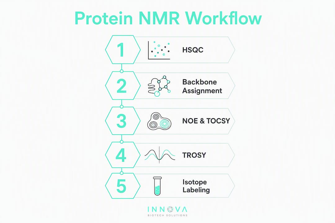
The 1H-¹⁵N HSQC (heteronuclear single-quantum coherence) is the universal starting point. It correlates each backbone amide ¹H with its directly bonded ¹⁵N, producing one peak per non-proline residue plus side-chain amides. A well-dispersed HSQC with sharp peaks tells you the protein is folded, monodisperse, and ready for further work. A collapsed, poorly dispersed spectrum tells you to fix the sample before investing in 3D experiments.

Infographic illustrating key NMR experiments for proteins

2D and 3D backbone assignment experiments

Once the HSQC looks good, triple-resonance 3D experiments assign each peak to a specific residue:

HNCA / HN(CO)CA: correlate each amide to its own Cα and the preceding residue's Cα, providing the sequential walk.
HNCACB / CBCA(CO)NH: add Cβ correlations, which are especially diagnostic for amino acid type (Cβ of Ser/Thr resonates upfield of most others).
HNCO / HN(CA)CO: carbonyl correlations, useful for secondary structure and RDC measurements.

These experiments require uniform ¹³C/¹⁵N labeling and are the standard route to backbone assignment for proteins up to ~25 kDa.

NOE and TOCSY for distance restraints

NOESY (nuclear Overhauser effect spectroscopy) is the workhorse for distance restraints. In 3D ¹³C- or ¹⁵N-edited NOESY experiments, cross-peak intensities are converted to upper-distance bounds (typically 5–6 Å) that drive structure calculation. TOCSY (total correlation spectroscopy) maps spin-system connectivity within a residue and is most useful for side-chain assignment.

Dynamics and dispersion experiments

R₁ and R₂ relaxation rates plus the heteronuclear ¹H-¹⁵N NOE characterize backbone dynamics on the ps-ns timescale.
CPMG relaxation dispersion and R₁ρ experiments quantify µs-ms exchange processes, revealing excited states and conformational switching.

Specialized methods for larger proteins

TROSY (transverse relaxation-optimized spectroscopy) exploits constructive interference between dipolar and CSA relaxation to narrow linewidths in large proteins. Paired with perdeuteration, it pushes the practical size ceiling substantially higher. Methyl-TROSY experiments on selectively labeled Ile, Leu, Val, and Met methyl groups extend this further, enabling studies of assemblies well beyond 100 kDa in favorable cases.

Pro Tip: For membrane proteins reconstituted in detergent micelles, the effective molecular weight is the protein-micelle complex, not the protein alone. A 20 kDa membrane protein in a 50 kDa micelle behaves like a 70 kDa system. Plan for TROSY from the start.

Why isotope labeling is non-negotiable for protein NMR

A natural-abundance protein spectrum is dominated by ¹H signals from every carbon and nitrogen in the molecule. For anything beyond a small peptide, the result is an unresolvable mess. Isotope enrichment with ¹³C and ¹⁵N is what makes multidimensional heteronuclear experiments possible and solves the assignment problem.

Choosing a labeling strategy

Uniform ¹⁵N labeling is the minimum for a backbone fingerprint (HSQC) and relaxation experiments. Cost is modest; expression in M9 minimal medium with ¹⁵NH₄Cl as the sole nitrogen source is standard in E. coli.

Uniform ¹³C/¹⁵N labeling is required for triple-resonance backbone assignment. Add [¹³C]-glucose to the M9 medium. This is the default for any protein under ~25 kDa where you plan a full assignment campaign.

Perdeuteration (²H, ¹³C, ¹⁵N) replaces most non-exchangeable protons with deuterium, dramatically reducing dipolar relaxation and sharpening lines in larger proteins. It is the prerequisite for TROSY-based experiments on proteins above ~30 kDa. The trade-off: deuterium slows back-exchange of amide protons, requiring careful refolding or extended incubation in H₂O buffer.

Selective methyl labeling (Ile-δ1, Leu/Val-pro-S, Met) in a perdeuterated background gives sharp, well-resolved methyl signals for large systems. This is the method of choice for assemblies, chaperones, and other high-molecular-weight targets.

Cell-free expression offers flexibility for toxic proteins and allows incorporation of non-natural amino acids or site-specific spin labels. Cost per milligram is higher than E. coli fermentation, but the ability to produce labeled protein that cannot be expressed in cells is often worth it.

Practical decision checklist

Protein < 15 kDa and you need only dynamics or binding data: uniform ¹⁵N is sufficient.
Protein 15–30 kDa and you want a full structure: uniform ¹³C/¹⁵N.
Protein 30–50 kDa: perdeuteration plus TROSY.
Protein > 50 kDa or a complex: selective methyl labeling in a perdeuterated background.
Toxic or insoluble in E. coli: cell-free expression with the appropriate isotope mix.

How to prepare a protein sample for NMR

Sample quality is the single biggest variable in how long an NMR campaign takes. A poorly prepared sample wastes instrument time; a well-prepared one makes every experiment faster.

Concentration and volume requirements

Tube type	Volume	Recommended concentration	Notes
Standard 5 mm	500–550 µL	0.1–1 mM	Routine; works for most experiments
Shigemi tube	260–300 µL	0.1–1 mM	Reduces sample volume; useful for precious proteins
Cryoprobe + Shigemi	260–300 µL	0.1–0.5 mM	Best sensitivity per milligram

Protein mass typically ranges from 2–30 mg depending on molecular weight, with approximately 10 mg typical for an 8–30 kDa protein in a standard 5 mm tube at 0.5 mM.

Statistic callout: For a 15 kDa protein at 0.5 mM in a 500 µL sample, you need roughly 3.75 mg of pure, labeled protein per NMR tube — and that same sample can be reused across multiple experiments since NMR is non-destructive.

Buffer and stability checklist

pH: Keep between 6.0 and 7.5 for amide exchange; lower pH slows exchange but may affect folding.
Salt: 50–150 mM NaCl is typical. High salt (> 300 mM) increases conductivity and reduces probe sensitivity, especially with cryoprobes.
Temperature: Most proteins are studied at 25–37°C; higher temperature improves tumbling but accelerates amide exchange.
Stabilizing additives: DTT or TCEP for cysteines; glycerol (up to 5%) for stability; protease inhibitors if degradation is a concern.
D₂O: Add 5–10% D₂O for the lock signal; do not use 100% D₂O unless you specifically want to observe only non-exchangeable protons.

For membrane proteins, the effective system size is the protein-detergent complex. Common choices include DPC, LPPG, and DHPC micelles for smaller membrane proteins; nanodiscs and bicelles are preferred when you need a more native-like bilayer environment and can tolerate the larger effective size. Protein stability prediction before committing to NMR sample prep can save weeks of troubleshooting.

What instruments and hardware do you need?

Magnet field strength, measured in MHz (the ¹H Larmor frequency), is the primary driver of both sensitivity and resolution. A 600 MHz spectrometer is a reasonable baseline for routine work on proteins up to ~25 kDa. A 800 or 900 MHz instrument improves resolution and sensitivity enough to matter for larger proteins, crowded spectra, and low-concentration samples.

Hardware that changes what you can do

Cryogenic probes cool the detection coil and preamplifier to ~20 K, reducing thermal noise. Cryogenic probes reduce thermal noise approximately 3–4-fold, which translates directly into shorter experiment times or lower required protein concentration.
Pulsed field gradients (PFGs) suppress artifacts and enable coherence selection in multidimensional experiments. They are standard on any modern research spectrometer.
TROSY-compatible hardware requires high-field magnets (≥ 600 MHz) and gradient-capable probes; the TROSY effect grows with field strength, so the investment in a 900 MHz instrument pays off specifically for large-protein work.
Benchtop spectrometers (60–100 MHz) are useful for quality control and teaching but lack the resolution and sensitivity for protein structure work.

Vendor and software ecosystem

Bruker and JEOL are the two primary manufacturers of high-field research NMR spectrometers. Bruker's TopSpin software handles instrument control, data acquisition, and basic processing and is the most widely used platform in academic and industrial NMR labs. JEOL instruments use their own Delta software environment.

Statistic callout: Higher magnetic field increases sensitivity in proportion to B₀^(3/2) for modern cryoprobe-equipped systems, meaning a jump from 600 to 900 MHz delivers roughly a 1.8-fold sensitivity gain per scan — before accounting for the additional resolution benefit.

What are the real strengths and limitations of protein NMR?

Unique strengths

Solution-state dynamics at atomic resolution: — NMR is the only technique that directly measures motion at every residue simultaneously, from fast side-chain flips to slow domain rearrangements.

Major limitations

Sensitivity: — NMR is inherently insensitive compared to fluorescence or mass spectrometry. Millimolar concentrations are often needed, which is demanding for proteins that aggregate or are difficult to express.

Comparing NMR modalities

Modality	Typical size range	Sensitivity / concentration	Best for
Solution NMR	5–50 kDa (routine: 5–25 kDa)	0.1–1 mM; moderate	Structure, dynamics, weak binding, IDPs
Solid-state NMR	No hard upper limit	Lower; requires more material	Membrane proteins, fibrils, insoluble assemblies
In-cell NMR	Small proteins (< 20 kDa typical)	Low; technically demanding	Intracellular environment, crowding effects

Pro Tip: The single most effective strategy for pushing past the 25 kDa ceiling is combining perdeuteration with TROSY-based triple-resonance experiments. Add selective methyl labeling if you need side-chain information. These two choices together have enabled de novo structures of proteins and complexes well beyond 50 kDa.

From FID to structure: software and data analysis

The processing and analysis pipeline has distinct stages, each with its own tools.

Processing: FID to spectrum

NMRPipe (Delaglio et al., NIH) is the standard for processing raw FID data into frequency-domain spectra. It handles apodization, zero-filling, Fourier transformation, phase correction, and baseline correction through scriptable pipelines. Most academic and industrial NMR labs use NMRPipe as the first step regardless of the spectrometer vendor. Bruker's TopSpin can also process data natively and is often used for quick checks directly on the instrument.

Visualization and assignment

Sparky (and its maintained fork, NMRFAM-Sparky) is the most widely used tool for interactive peak picking and resonance assignment. It displays 2D and 3D spectra, allows manual and semi-automated peak picking, and tracks assignment progress across experiments.

CcpNmr Analysis (from the Collaborative Computational Project for NMR) is a more integrated platform that handles the full assignment workflow, stores data in a standardized CCPN data model, and exports restraint files directly to structure calculation packages. For projects that will go all the way to a deposited structure, CcpNmr's data model is the cleaner choice.

CYANA uses torsion-angle molecular dynamics with NOE-derived distance restraints and dihedral angle restraints to calculate an ensemble of structures. It includes automated NOE assignment (CANDID/FLYA) that dramatically reduces manual work.
Xplor-NIH (NIH) performs simulated annealing and refinement in Cartesian or torsion-angle space, incorporating NOEs, RDCs, chemical shift restraints, and PRE data. It is the standard for final refinement before PDB deposition.

Automation and modern approaches

Non-uniform sampling (NUS) reduces experiment time by acquiring only a fraction of the traditional time-domain grid, then reconstructing the full spectrum. Automated assignment pipelines (FLYA in CYANA, PINE from NMRFAM) can assign backbone resonances with minimal manual intervention for well-behaved proteins, cutting weeks of analysis to days.

How NMR supports drug discovery and fragment screening

NMR's role in drug discovery is most powerful at the earliest stages, where other methods struggle with weak binders.

Fragment screening and hit identification

Fragment-based drug discovery (FBDD) relies on detecting millimolar-affinity binders that would be invisible to most assays. NMR handles this directly. Ligand-observed experiments (STD, WaterLOGSY, ¹H T₂ filtering) screen mixtures of fragments against a target protein and flag binders by changes in ligand relaxation or NOE. Protein-observed HSQC titrations then map exactly which residues are perturbed, identifying the binding site at atomic resolution.

STD (saturation transfer difference): Fast, requires only unlabeled protein, screens mixtures of up to 10–20 compounds per experiment.
WaterLOGSY: Complementary to STD; useful for confirming weak binders and distinguishing specific from non-specific binding.
HSQC titration: Protein-observed; requires ¹⁵N-labeled protein; gives site-specific binding information and a Kd estimate from the titration curve.
CPMG relaxation dispersion: Quantifies exchange kinetics for bound and free states, giving kon and koff in favorable cases.

From hit to lead with NMR

Once a fragment hit is confirmed, NMR guides optimization. Chemical shift perturbation maps define which residues contact the ligand, which informs where to grow the fragment. NMR can map binding sites for millimolar-affinity ligands and guide fragment linking to produce tighter leads. The same HSQC titration experiment run on each analog in a series tells you immediately whether a modification improved binding (larger shift, slower exchange) or disrupted it.

NMR also detects allostery directly: a ligand binding at site A that shifts residues at site B, 20 Å away, is visible in the HSQC perturbation map. No docking model is needed to see it. This makes NMR uniquely suited to identifying cryptic and allosteric sites that only open transiently.

Pro Tip: Run a ligand-observed STD screen first to triage your fragment library cheaply, then invest in protein-observed HSQC titrations only for confirmed hits. This two-stage approach cuts instrument time by 60–80% compared to running HSQC titrations on every compound.

How long does a protein NMR campaign take, and what does it cost?

Typical timelines and protein requirements

Task	Protein needed	Instrument time	Analysis time
¹H-¹⁵N HSQC fingerprint	2–5 mg (¹⁵N-labeled)	30 min–2 h	1–2 h
Backbone assignment (< 20 kDa)	10–15 mg (¹³C/¹⁵N)	3–7 days	2–4 weeks
Full structure determination	15–30 mg (¹³C/¹⁵N ± ²H)	2–4 weeks	2–4 months
Fragment screen (ligand-observed)	1–5 mg (unlabeled)	1–3 days	1–2 weeks
Dynamics (R₁/R₂/NOE suite)	5–10 mg (¹⁵N)	2–5 days	1–3 weeks

Sample volumes run 500–550 µL for standard 5 mm tubes and 260–300 µL for Shigemi tubes, with protein mass in the 2–30 mg range depending on molecular weight.

Cost drivers

Instrument time at academic shared facilities in the United States typically runs $20–80/hour for 600–800 MHz spectrometers, though rates vary widely by institution. Isotope-labeled media (¹⁵N, ¹³C) add $200–800 per liter of expression culture. Personnel time for assignment and structure calculation is often the largest cost: a full backbone assignment for a 20 kDa protein takes an experienced spectroscopist 2–4 weeks of focused analysis.

Planning checklist

Confirm protein stability at NMR concentrations (0.5 mM, 25–37°C, 24–72 h) before booking instrument time.
Run a 1D ¹H spectrum first; if it looks like noise, fix the sample.
Use Shigemi tubes when protein is scarce; the sensitivity-per-milligram gain is real.
For structure determination, budget at least 15 mg of ¹³C/¹⁵N-labeled protein before you start.
Consider outsourcing to a shared NMR facility or a contract research organization if in-house access is limited; many U.S. universities offer external access rates.

How NMR data integrates with computational workflows

NMR-derived restraints and dynamics data are not just outputs for publication. They are inputs that make computational models more accurate and docking predictions more reliable.

Integration points

NOE-derived distance restraints refine homology models — When a crystal structure is unavailable, NMR restraints can correct loop geometries and side-chain packing in a homology model before docking.

A practical workflow example

A fragment hit identified by HSQC titration produces a CSP map showing 12 perturbed residues clustered on one face of the protein. That map is passed to a docking pipeline as a set of binding-site constraints. The docking run generates 1,000 poses; only those placing the fragment within 5 Å of all 12 perturbed residues are retained. The surviving poses are then ranked by a scoring function, and the top 5 are passed to a short MD simulation for stability assessment. This kind of NMR-guided virtual screening reduces the docking search space by an order of magnitude and dramatically improves hit quality.

Pro Tip: When handing NMR data to a computational team, deliver the CSP map as a ranked residue list with Δδ values, not just a figure. Include the raw HSQC overlays and the assignment table. A computational modeler needs the numbers, not a color-coded picture.

Innovabiotech's protein design and computational modeling services are built to receive exactly this kind of NMR-derived input, integrating experimental restraints into structure-based design and hit-to-lead optimization pipelines.

Key Takeaways

Protein NMR is the only technique that simultaneously reports atomic-resolution structure, site-specific dynamics across multiple timescales, and weak-affinity interactions in solution, making it irreplaceable for IDPs, fragment screening, and allostery studies.

Point	Details
Start with an HSQC	The 1H-¹⁵N HSQC fingerprint is the first experiment for any new protein; it confirms folding and sample quality before committing to longer campaigns.
Isotope labeling is mandatory	Uniform ¹⁵N/¹³C is required for backbone assignment; perdeuteration plus TROSY extends the practical size range beyond 25 kDa.
Sample requirements are specific	Plan for 0.1–1 mM protein in 260–550 µL; approximately 10 mg of labeled protein is typical for an 8–30 kDa target.
NMR detects what other methods miss	Relaxation-dispersion experiments reveal excited states at ~1% population, and CSP mapping detects millimolar-affinity ligands invisible to most assays.
Innovabiotech bridges NMR and computation	Innovabiotech integrates NMR-derived restraints and CSP maps into docking, protein design, and hit-to-lead optimization workflows for pharma and biotech clients.

NMR's unique value, from where I sit

NMR has a reputation for being difficult, and that reputation is earned. But the difficulty is almost never in the physics or the hardware. It is in the protein.

The real challenge is that proteins are not static objects. They sample conformational ensembles across timescales that span 15 orders of magnitude, from sub-nanosecond methyl rotations to minute-scale domain rearrangements. Interpreting NMR data requires integrating spatial and temporal information to build biologically meaningful models, and that is genuinely hard. A crystal structure gives you one snapshot. NMR gives you a movie, and movies are harder to interpret than photographs.

What gets underestimated is how much that difficulty pays off. The excited states that CPMG dispersion experiments reveal are not curiosities. They are often the states that bind drugs, catalyze reactions, or transmit allosteric signals. A protein that looks rigid in a crystal structure may be sampling an open conformation 2% of the time, and that 2% is where the biology happens. NMR is the only technique that sees it directly.

The other thing practitioners underestimate is how well NMR and computation complement each other. A CSP map from a 2-hour HSQC titration experiment can cut a docking campaign from weeks to days by eliminating 90% of the search space. The experimental data does not replace the computation; it makes the computation trustworthy. That integration is where the real efficiency gains are, and it is still underused in most drug-discovery pipelines.

Innovabiotech's computational services for NMR-driven projects

For research teams that have NMR data and need to move it into a design or optimization pipeline, the bottleneck is rarely the data itself. It is the translation from experimental observables to a computational model that a medicinal chemist or protein engineer can act on.

Innovabiotech

Innovabiotech specializes in exactly that translation. The team takes NMR-derived inputs (CSP maps, NOE restraints, dynamics profiles, ensemble coordinates) and integrates them into structure-based protein design and hit-to-lead optimization workflows. Services include NMR-guided docking with binding-site constraints, peptide design and affinity optimization using NMR-mapped interaction surfaces, virtual screening with NMR-defined pharmacophores, and de novo peptide design informed by experimental binding data. Every project is handled under a confidential workflow with clear milestone deliverables, so pharma and biotech clients know exactly what they are getting and when.

If you have NMR data and need a computational team that knows how to use it, contact Innovabiotech to discuss your project.

Point	Details
Foundational theory	Poulsen's introduction and the UCSB NMR theory pages cover the physics and assignment strategies for beginners.
Dynamics methods	The ACS Analytical Chemistry review and the PMC dynamics article are the standard references for relaxation and dispersion experiments.
Drug discovery applications	The ScienceDirect "Boundless opportunities" review covers fragment screening, IDPs, and in-cell NMR comprehensively.
Software and tools	CcpNmr (assignment), NMRPipe (processing), Sparky (visualization), CYANA and Xplor-NIH (structure calculation) are the standard pipeline.
Sample planning	The MSU sample requirements page gives practical volumes and protein mass estimates for common tube types and molecular-weight ranges.

FAQ

What is NMR spectroscopy of proteins in simple terms?