

TL;DR:
- Monte Carlo simulation quantifies uncertainty by repeatedly sampling from biological parameter distributions to explore system behaviors. It excels when parameters are uncertain, high-dimensional, and outputs require confidence intervals, informing decisions in drug development and molecular modeling.
A Monte Carlo simulation in biology is a computational method that uses repeated random sampling from defined probability distributions to quantify uncertainty and explore possible system behaviors across a biological model. Instead of solving a single deterministic equation, you run the model thousands of times, each time drawing slightly different parameter values, and collect the resulting output distribution. That distribution tells you not just what is likely, but how confident you should be, and where your model is most sensitive to uncertainty.
Biologists reach for Monte Carlo when three conditions converge:
- Uncertainty is real and measurable. Parameters like drug clearance rates, enzyme Km values, or ion channel gating probabilities are never known exactly; Monte Carlo propagates that uncertainty honestly.
- The solution space is high-dimensional. Metabolic networks, protein conformational ensembles, and multi-drug PK/PD models have too many interacting variables for any closed-form solution.
- You need a distribution, not a point estimate. Confidence intervals, credible intervals, and ensemble outputs are the currency of modern biological decision-making.
Typical use cases span PK/PD dose-uncertainty modeling, protein folding conformational sampling, metabolic network analysis with the COBRA framework, ion channel transport, and radiobiology track-structure simulations. Innovabiotech applies these methods directly in drug-discovery pipelines, from hit identification through lead optimization.
Table of Contents
- What is Monte Carlo simulation in biology, and why does it work statistically?
- When does Monte Carlo add the most value in biological research?
- Which Monte Carlo variants do biologists actually use?
- How to set up and run a Monte Carlo simulation for a biological project
- A worked example: enzyme kinetics uncertainty with Monte Carlo
- What tools and software support Monte Carlo work in biology?
- What are the real strengths and limits of Monte Carlo in biological models?
- How should you validate and report Monte Carlo results?
- How Innovabiotech applies Monte Carlo in drug-discovery projects
- Key Takeaways
- Why the way most researchers use Monte Carlo is subtly wrong
- Innovabiotech brings Monte Carlo modeling to your drug-discovery pipeline
- Useful sources and further reading
- FAQ
What is Monte Carlo simulation in biology, and why does it work statistically?
The core idea is straightforward: replace an intractable integral or an analytically unsolvable system with an empirical average over many random samples. If you draw N samples from the input distributions and run your model each time, the sample average of the outputs converges to the true expected value as N grows. That is the Law of Large Numbers at work, and it is why Monte Carlo is so broadly applicable even when the underlying biology is messy and nonlinear.
A conceptual sketch of the process:
- Inputs: Define each uncertain parameter (e.g., drug absorption rate ka, volume of distribution Vd) as a probability distribution (normal, log-normal, uniform, or empirically derived).
- Sampler: Draw one value for each parameter from its distribution.
- Model run: Plug those values into your biological model (ODE, agent-based, spatial grid) and record the output of interest (e.g., peak plasma concentration Cmax).
- Repeat N times: Collect all N outputs into a histogram.
- Analyze: Read off the mean, median, 95th percentile, and credible intervals directly from that histogram.
The bootstrap is a closely related technique: instead of sampling from a parametric distribution, you resample with replacement from your actual experimental dataset to form synthetic datasets and estimate parameter confidence regions. Bootstrap is especially useful when you cannot assume a distribution shape, and multiplicative Monte Carlo variants help enforce positivity for parameters that must stay above zero (enzyme concentrations, rate constants).
Diagram description: Picture a funnel. At the top, five input sliders each show a distribution curve. The funnel runs thousands of virtual "worlds" in parallel. At the bottom, a single histogram emerges, showing the spread of possible outcomes. The width of that histogram is your uncertainty.
Pro Tip: For most biological models, 1,000–10,000 samples is a reasonable starting range. Run 1,000 first and check whether the output mean and variance have stabilized; if they are still shifting noticeably between runs, double the sample count. Computational cost scales roughly linearly with sample count for simple ODE models, so there is rarely a reason to start at 100,000.

When does Monte Carlo add the most value in biological research?
The honest answer: whenever your model has uncertain parameters and the output distribution matters more than a single best-fit prediction. Here are the principal application areas where Monte Carlo methods in biology consistently outperform deterministic approaches.
- PK/PD and dose uncertainty. Drug absorption, distribution, metabolism, and excretion parameters vary across patients. Monte Carlo propagates that variability through a PK model to produce a distribution of predicted plasma concentrations, letting you set dose ranges that keep most patients within a therapeutic window while avoiding toxicity.
- Protein folding and conformational ensembles. Rather than finding a single lowest-energy structure, Monte Carlo sampling explores the conformational space and produces an ensemble of plausible structures. That ensemble is more biologically honest than a single snapshot and directly informs binding-site analysis.
- Disease progression models. Stochastic patient-level models use Monte Carlo to simulate heterogeneous disease trajectories across a virtual population, generating survival curves and treatment-response distributions that feed directly into clinical trial design.
- Metabolic network sampling with COBRA. In genome-scale metabolic models, the feasible solution space is a high-dimensional polytope. Monte Carlo sampling within the COBRA framework draws representative flux states from that polytope, revealing which metabolic routes are robust and which are fragile under different conditions.
- Ion transport and ion channels. Stochastic gating models for ion channels use Monte Carlo to simulate the probabilistic opening and closing of individual channels, producing realistic membrane current distributions that match patch-clamp recordings far better than deterministic conductance models.
- Radiobiology and DNA damage (track-structure MC). Particle-based Monte Carlo simulates the physical tracks of ionizing radiation particles through biological tissue, scoring DNA strand breaks and clustered damage sites. This approach is essential for understanding radiation therapy dose-response at the molecular level.
A practical payoff: in PK/PD work, the output distribution directly tells you which dose levels carry unacceptable toxicity risk for the 95th-percentile patient, letting you design a clinical trial with a tighter, evidence-based dose range before a single patient is enrolled.
Which Monte Carlo variants do biologists actually use?
Not all Monte Carlo is the same algorithm. The biological problem you are solving determines which variant to reach for.
| Variant | Time evolution | Key inputs | Computational cost | Typical biological use |
|---|---|---|---|---|
| Classical Monte Carlo | Equilibrium sampling | Parameter distributions, model equations | Low–moderate | PK/PD uncertainty, conformational ensembles |
| Bootstrap / resampling | None (data-driven) | Experimental dataset | Low | Parameter confidence intervals, data-limited models |
| Gillespie / SSA | Explicit, event-driven | Reaction rates, species counts | Moderate | Gene expression noise, small-molecule reaction networks |
| Kinetic Monte Carlo (kMC) | Explicit, transition-based | Rate constants, state definitions | Moderate–high | Enzyme kinetics, protein-ligand dynamics, regulatory networks |
| Particle-based (track-structure) | Explicit, spatial | Particle physics cross-sections, geometry | High | Radiobiology, DNA damage, ion transport |
When to use which:
- SSA / Gillespie: Pick this when molecule counts are small (tens to hundreds of molecules) and stochastic fluctuations matter, such as in gene regulatory circuits or early-stage viral infection models.
- Kinetic Monte Carlo (kMC): Use kMC when you need to model transitions across time and length scales explicitly, such as enzyme conformational changes, receptor-ligand binding kinetics, or multi-step signaling cascades. For rare events (slow folding, infrequent binding), rejection-free kMC algorithms are essential; naive brute-force sampling will miss those events entirely.
- Particle-based / track-structure: Reserve for spatial problems where the physical path of a particle through tissue matters, primarily radiation biology.
- Bootstrap: Default choice when you have experimental data but cannot justify a parametric distribution assumption.
- Hybrid models: Combining kMC with differential-equation approaches lets you capture multi-scale phenomena, such as membrane-shape dynamics coupled with receptor-ligand kinetics, that no single method handles cleanly.
How to set up and run a Monte Carlo simulation for a biological project
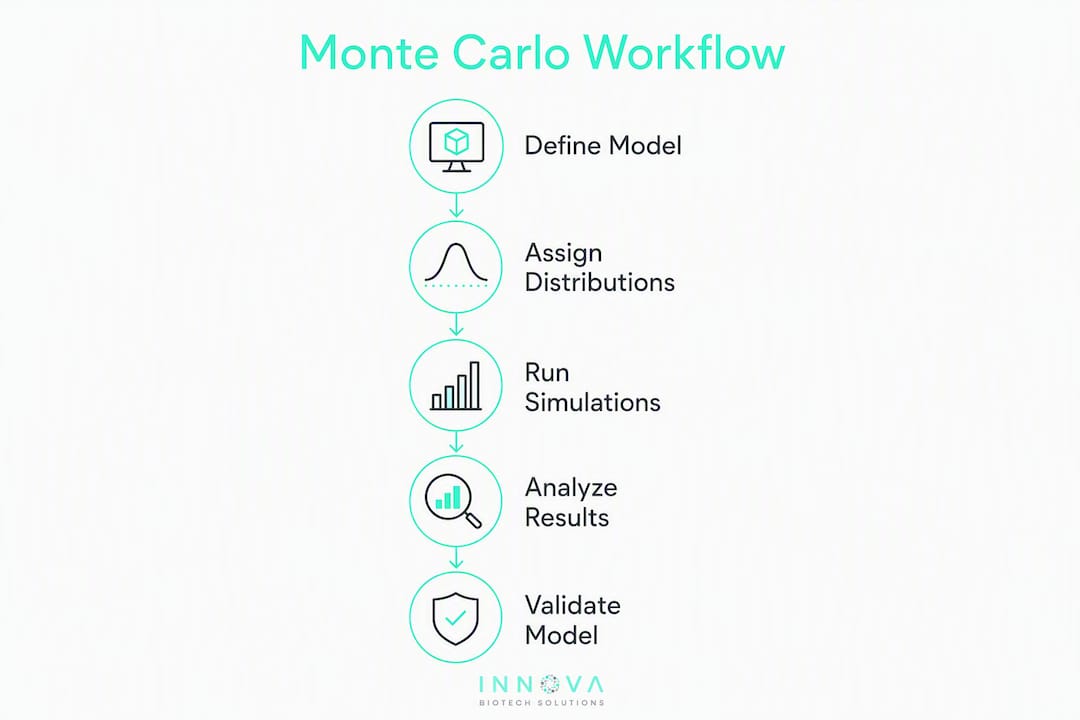
A structured workflow prevents the most common failure modes: poorly chosen distributions, insufficient samples, and results that cannot be reproduced.
- Define the biological question precisely. What output do you need a distribution for? (e.g., "What is the likely range of Cmax for a 10 mg dose across a patient population?") A vague question produces an uninterpretable output distribution.
- Choose your model form. ODE systems work for well-mixed compartments (PK/PD, enzyme kinetics). Agent-based models suit spatial or population-level heterogeneity. Spatial grids or particle trackers suit radiation or diffusion problems.
- Identify uncertain inputs and assign distributions. For each uncertain parameter, choose a distribution based on prior data or literature. Log-normal is common for biological rate constants (they are always positive and often span orders of magnitude). Uniform distributions are appropriate when you only know bounds.
- Choose your Monte Carlo variant. Use the table in the previous section as your guide.
- Implement the sampler. In Python,
numpy.randomorscipy.statshandles most parametric distributions. For Bayesian inference, PyMC provides a full probabilistic programming framework. - Run the ensemble. Start with N = 1,000. Record every output of interest, not just the mean.
- Analyze output distributions. Compute mean, median, 5th and 95th percentiles. Plot histograms and cumulative distribution functions. Check for bimodality or heavy tails, which often signal a structural model issue.
- Run convergence checks. Plot the running mean and running variance as a function of N. If both have stabilized, you have enough samples. If variance is still drifting at N = 10,000, either your model is highly nonlinear or your distributions are too wide.
- Perform sensitivity analysis. Vary one input distribution at a time (or use Sobol indices for a formal global sensitivity analysis) to identify which parameters drive the most output variance. Those are the parameters worth measuring more precisely in the lab.
Pro Tip: Assign parameter distributions before you look at the output. Choosing distributions to match a desired output is a form of circular reasoning that invalidates the uncertainty estimate entirely. Document your prior choices and their justification in a methods log from day one.
Runtime and hardware: for ODE-based PK models with N = 10,000 samples, a modern laptop finishes in seconds to minutes. For spatial particle-track simulations or large agent-based models, expect hours to days on a workstation or cluster.
A worked example: enzyme kinetics uncertainty with Monte Carlo
The problem. You have measured the Michaelis-Menten parameters Km and Vmax for an enzyme of interest, but each measurement carries experimental uncertainty. You want to know the likely range of reaction velocity v at a substrate concentration [S] = 50 µM.

The model. Michaelis-Menten: v = Vmax × [S] / (Km + [S])
Input table:
| Parameter | Distribution | Mean | SD / Bounds |
|---|---|---|---|
| Vmax (µmol/min) | Log-normal | 10.0 | σ = 0.2 (log scale) |
| Km (µM) | Log-normal | 30.0 | σ = 0.3 (log scale) |
| [S] (µM) | Fixed | 50.0 | — |
Pseudocode (Python-style):
import numpy as np

N = 10000
Vmax_samples = np.random.lognormal(mean=np.log(10.0), sigma=0.2, size=N)
Km_samples   = np.random.lognormal(mean=np.log(30.0), sigma=0.3, size=N)
S = 50.0

v_samples = Vmax_samples * S / (Km_samples + S)

print(f"Mean v:       {np.mean(v_samples):.2f} µmol/min")
Expected output. The histogram of v_samples will be right-skewed (because both inputs are log-normal).
Interpreting the results:
- A narrow histogram means your uncertainty in Km and Vmax does not strongly affect predictions at this substrate concentration. You can trust point-estimate kinetics for this condition.
- A wide or skewed histogram means experimental uncertainty in one or both parameters is driving meaningful variability in predicted velocity. That is a signal to invest in tighter Km measurements before using this enzyme in a design decision.
- To check robustness: widen the log-normal σ values by 50% and rerun. If the credible interval doubles, your conclusions are fragile. If it barely changes, they are stable.
For protein stability applications, the same framework applies: sample over uncertain thermodynamic parameters and collect a distribution of predicted stability scores rather than a single ΔG estimate.
What tools and software support Monte Carlo work in biology?
The ecosystem is mature. The right tool depends on your problem type and how much you want to build from scratch.
| Tool / Library | Best for | Quick-start effort |
|---|---|---|
| Python (NumPy / SciPy) | General sampling, PK/PD, enzyme kinetics | Low |
| PyMC / NumPyro | Bayesian inference, parameter estimation | Moderate |
| MATLAB | ODE-based PK/PD, systems biology | Low–moderate |
| COBRA Toolbox (MATLAB/Python) | Metabolic network sampling | Moderate |
| COPASI | Stochastic kinetics, SSA / Gillespie | Low |
| StochPy | Stochastic simulation in Python | Low |
| BioNetGen | Rule-based stochastic reaction networks | Moderate |
| BioMOCA | Ion transport / ion channel Monte Carlo | Moderate–high |
A few notes on specific tools:
- COPASI is the fastest path to a working Gillespie simulation for a biochemical reaction network. Its GUI lets you define reactions, assign stochastic parameters, and run SSA without writing code.
- BioMOCA (Bio Monte Carlo for ion channels) is a specialized particle-based simulator developed for ion transport through biological channels. It models ion trajectories explicitly and is the standard tool for nanoscale ion channel studies.
- COBRA Toolbox is the standard for metabolic network Monte Carlo sampling. Using an established toolbox rather than building a custom sampler avoids subtle errors in high-dimensional polytope sampling and improves reproducibility.
- PyMC is worth learning if you plan to do any Bayesian parameter estimation. It handles posterior sampling via MCMC (Markov Chain Monte Carlo), which is the Bayesian cousin of the classical Monte Carlo approaches described here.
For computational protein modeling, Python-based sampling pipelines paired with structure-prediction tools give you the most flexibility for conformational ensemble work.
Tutorials and starting points: the COPASI website hosts worked examples for stochastic kinetics; the PyMC documentation includes a pharmacokinetics notebook; BioNetGen's GitHub repository contains rule-based stochastic network examples. For metabolic sampling, the COBRA Toolbox documentation walks through flux sampling step by step.
What are the real strengths and limits of Monte Carlo in biological models?
Strengths:
- Handles nonlinearity naturally. No Taylor-series approximations, no normality assumptions.
- Scales to high-dimensional parameter spaces where analytical uncertainty propagation fails.
- Produces full output distributions, not just means and standard deviations.
- Flexible enough to work with any model form: ODEs, agent-based, spatial, hybrid.
- Directly supports decision-making by quantifying tail risks (e.g., probability of toxicity at a given dose).
Limitations and common pitfalls:
- Computational cost. Complex models (large agent-based, spatial particle-track) can require days of compute time. More samples do not fix a flawed model; they just give you a more precise wrong answer.
- Garbage-in, garbage-out on distributions. If you assign a normal distribution to a parameter that is physically bounded below zero, you will sample impossible values. Use log-normal or truncated distributions for rate constants and concentrations.
- Overfitting to scarce data. Fitting distribution parameters to a handful of experimental measurements and then treating the resulting Monte Carlo output as a reliable uncertainty estimate is circular. The uncertainty in your distribution parameters is itself uncertain.
- Sampling bias. In high-dimensional spaces, naive random sampling concentrates in the corners of the parameter space. Quasi-random (Sobol, Halton) sequences or Latin hypercube sampling give better coverage with fewer samples.
- Ignoring model structural uncertainty. Monte Carlo quantifies parameter uncertainty within a fixed model structure. If the model itself is wrong (wrong reaction mechanism, missing pathway), no amount of sampling will reveal that.
Key insight: The most dangerous Monte Carlo result is a narrow, confident-looking output distribution produced by a model whose structural assumptions were never validated against experimental data. Convergence of the sampler is not the same as correctness of the model. Always compare your simulation outputs to at least one independent experimental dataset before drawing conclusions.
How should you validate and report Monte Carlo results?
Reproducibility is where Monte Carlo work most often falls short in published biology papers. A checklist:
Validation:
- Calibrate model outputs against at least one independent experimental dataset not used to set the input distributions.
- Run convergence diagnostics: plot running mean and variance versus N; report the N at which both stabilized.
- Perform sensitivity analysis and report which parameters drive the most output variance.
- Compare Monte Carlo outputs to a simpler model (e.g., a deterministic ODE with best-fit parameters) to confirm the stochastic model adds genuine predictive value.
Reporting template elements:
- State all model assumptions explicitly (compartment structure, reaction mechanism, independence of parameters).
- Report input distributions: distribution type, mean, variance, and the source (literature, experimental fit, expert prior).
- Report number of runs (N), random seed, and software version.
- State convergence criteria used.
- Report credible intervals (e.g., 95% CI) alongside means; never report only the mean.
- Present uncertainty visually: histograms, credible interval bands on time-course plots, or violin plots for parameter posteriors.
Reproducible sharing: version-control your simulation code (Git), pin software dependencies (a requirements.txt or conda environment file), and share the code and seed alongside the paper. Docker containers are increasingly standard for complex multi-tool pipelines. For drug sensitivity prediction workflows that combine Monte Carlo with machine learning, containerized environments are practically mandatory for reproducibility.
Statistic callout: Peer-reviewed guidance consistently emphasizes that alignment of model mechanisms with known biology matters more than simply increasing sample size. A well-validated model with N = 1,000 samples is more defensible than a poorly validated one with N = 1,000,000.
How Innovabiotech applies Monte Carlo in drug-discovery projects
Innovabiotech's computational biology team integrates Monte Carlo uncertainty quantification directly into drug-discovery pipelines, from early virtual screening through hit-to-lead optimization.
Pipeline overview:
- Problem definition and data curation. Define the biological target, collect experimental kinetic or binding data, and identify uncertain parameters.
- Model building. Construct a PK/PD, enzyme kinetics, or protein-ligand binding model appropriate to the project stage.
- Monte Carlo sampling and uncertainty quantification. Run ensemble simulations to produce output distributions for key decision variables (predicted Cmax, binding affinity range, metabolic flux robustness).
- Prioritized experiments. Use sensitivity analysis outputs to identify which parameters most reduce output uncertainty when measured more precisely, directly informing which assays to run next.
- Hit-to-lead optimization. Feed uncertainty-quantified predictions into hit-to-lead workflows to rank candidate compounds by predicted efficacy and safety margin, not just by a single point-estimate score.
Deliverables from a typical Monte Carlo engagement:
- Validated simulation code with documented assumptions and reproducible random seeds
- Sensitivity analysis report identifying the top uncertainty drivers
- Prioritized assay list derived from sensitivity outputs
- Uncertainty visualization package (histograms, credible interval plots, tornado diagrams)
- Written methods section suitable for inclusion in a regulatory submission or publication
All client data and model details are handled under confidentiality agreements, and all deliverables are version-controlled and containerized for full reproducibility. For applied examples of how computational modeling informs target prioritization, see Innovabiotech's work on VDAC1 inhibition.
Key Takeaways
Monte Carlo simulation in biology is most powerful when you need a full output distribution, not a point estimate, and when parameter uncertainty or stochastic dynamics are central to the biological question.
| Point | Details |
|---|---|
| Use Monte Carlo for uncertainty | When parameters are uncertain and you need confidence intervals, not just a best-fit value. |
| Match variant to problem | Use SSA/Gillespie for small molecule counts, kMC for event-driven kinetics, bootstrap for data-limited cases. |
| Validate before concluding | Convergence of the sampler does not equal correctness; always calibrate against independent experimental data. |
| Report distributions, not just means | Always report credible intervals, input distributions, N, and random seed for reproducibility. |
| Innovabiotech for applied work | Innovabiotech delivers Monte Carlo-based uncertainty quantification and sensitivity analysis for drug-discovery and protein-engineering projects. |
Why the way most researchers use Monte Carlo is subtly wrong
Monte Carlo is one of those methods that looks straightforward until you have used it on a real biological dataset and watched it produce a beautifully precise answer to the wrong question.
The most common mistake is not a coding error. It is treating the choice of input distributions as a formality rather than a scientific claim. When you assign a log-normal distribution with a particular mean and variance to an enzyme's Km, you are making a hypothesis about the population of possible Km values. If that hypothesis is wrong, the output distribution is wrong, regardless of how many samples you ran or how clean your convergence plots look. The simulation will converge. It will just converge to a confident mischaracterization of reality.
The second underappreciated issue is the gap between parameter uncertainty and model structural uncertainty. Monte Carlo handles the first beautifully. It does nothing about the second. A model that assumes Michaelis-Menten kinetics for an enzyme that actually shows cooperative behavior will produce a tidy output distribution that is systematically biased. More samples will not fix it.
The practical implication: before you run a single Monte Carlo sample, spend time on model validation. Compare your deterministic best-fit model to experimental data. Check residuals. Ask whether the model structure is biologically plausible. That work is less exciting than watching a histogram emerge, but it is what separates a defensible result from a compelling-looking artifact.
One more thing worth saying directly: simulations complement experiments; they do not replace them. The output of a Monte Carlo run is a hypothesis about what the biology might be doing, expressed probabilistically. The experiment is still the test. The most productive use of Monte Carlo in a lab setting is to run simulations before designing an experiment, use the sensitivity analysis to identify which measurements will most reduce your uncertainty, and then go measure those things. That iterative loop, simulation informing experiment informing simulation, is where the real value lives.
Innovabiotech brings Monte Carlo modeling to your drug-discovery pipeline
Running Monte Carlo simulations well requires more than a Python script. It requires a validated model, defensible input distributions, a sensitivity analysis that actually guides experimental decisions, and deliverables your team can reproduce and publish. That is exactly what Innovabiotech provides.

Innovabiotech's computational biology team in San Francisco builds custom Monte Carlo uncertainty quantification workflows for PK/PD modeling, enzyme kinetics, protein-ligand binding, and metabolic network analysis. Every engagement delivers validated, version-controlled code, a sensitivity report, and uncertainty visualizations ready for regulatory submissions or peer-reviewed publications. For projects at the protein or peptide level, the team's protein design services integrate Monte Carlo conformational sampling directly into the design-and-optimization loop.
If your project involves uncertain parameters, stochastic dynamics, or a decision that depends on knowing the full range of possible outcomes rather than a single best guess, reach out to Innovabiotech at innovabiotech.com to discuss a scoped engagement.
Useful sources and further reading
The sources below are selected for depth and accessibility. Peer-reviewed reviews are the right citation for Monte Carlo methods in published work; tool documentation is the right starting point for implementation.
| Source | Best for | Type |
|---|---|---|
| Applications of Monte Carlo Methods in Biology, Medicine and Other Fields of Science (NCBI Bookshelf) | Conceptual grounding, biological applications overview | Review / textbook chapter |
| Monte Carlo sampling within COBRA (PMC) | Metabolic network sampling, COBRA framework | Peer-reviewed article |
| Kinetic Monte Carlo in Biophysics and Systems Biology (PMC) | kMC theory, enzyme kinetics, regulatory networks | Peer-reviewed article |
| Applications of Monte Carlo Simulation in Modelling of Biochemical Processes (PubMed) | Bootstrap and multiplicative MC for biochemical models | Peer-reviewed article |
| Impact of DNA Geometry and Scoring on Monte Carlo Track-Structure (PMC) | Radiobiology, DNA damage, particle-based MC | Peer-reviewed article |
| Kinetic Monte Carlo Simulation in Biophysics (ResearchGate) | Rare-event kMC, rejection-free algorithms | Peer-reviewed article |
| Monte Carlo in Biotechnology (LabXchange) | Introductory tutorial, drug development context | Tutorial / educational |
Annotation notes:
- For conceptual grounding, start with the NCBI Bookshelf review and the LabXchange tutorial.
- For implementation, the COBRA Toolbox documentation, COPASI user manual, and PyMC documentation are the most practical starting points.
- For peer-reviewed citation in a publication, use the PMC and PubMed articles above; they are indexed and carry DOIs.
- Always cite the original peer-reviewed source when reporting Monte Carlo results in a paper, not a tutorial or blog post.
FAQ
What is Monte Carlo simulation in simple terms?
Monte Carlo simulation runs a model thousands of times, each time using randomly sampled input values, and collects the results into a distribution. The distribution shows you the range of likely outcomes and how confident you can be in any single prediction.
What is Monte Carlo simulation in science?
In science, Monte Carlo simulation is a numerical method for quantifying uncertainty and exploring complex system behaviors when analytical solutions are unavailable. It is used across biology, physics, chemistry, and medicine to propagate parameter uncertainty and estimate output distributions from stochastic models.
What is Monte Carlo simulation of DNA?
Monte Carlo simulation of DNA typically refers to particle-based track-structure simulations that model how ionizing radiation interacts with DNA geometry, scoring strand breaks and clustered damage sites. These simulations are central to radiobiology research and radiation therapy dosimetry.
Can ChatGPT run a Monte Carlo simulation?
ChatGPT can write Python or MATLAB code for a Monte Carlo simulation, but it does not execute the simulation itself. You run the generated code in your own environment using tools like NumPy, SciPy, or COPASI to produce actual results.
Which software is best for Monte Carlo simulation in biology?
The right tool depends on the problem: COPASI for stochastic reaction kinetics (Gillespie/SSA), the COBRA Toolbox for metabolic network sampling, PyMC for Bayesian parameter estimation, and BioMOCA for ion channel transport simulations. Python with NumPy and SciPy covers most general-purpose PK/PD and enzyme kinetics cases.