
Protein–ligand docking predicts the bound pose of a small molecule inside a protein binding site and returns a rapid, approximate score of binding affinity, making it the workhorse of structure-based virtual screening, SAR triage, and hit-to-lead prioritization. The method does not replace experimental measurement, but it narrows a library of thousands (or millions) of compounds to a tractable shortlist before any assay runs.
Three use cases drive most docking projects:
- Virtual screening (VS): rank a large compound library by predicted affinity to identify hits from scratch.
- SAR and hit-to-lead triage: rationalize why analogs differ in potency and guide the next synthesis round.
- Mechanistic hypothesis generation: propose binding modes to design mutagenesis experiments or explain selectivity.
The canonical pipeline, in brief:
- Prepare the receptor structure (repair, protonate, define the binding box).
- Prepare the ligand library (enumerate tautomers, protonation states, stereoisomers, conformers).
- Run the docking search (sampling algorithm places and scores poses).
- Post-filter and rescore top poses (consensus scoring, MM-GBSA, or FEP for leads).
Every section below unpacks one of those steps in the depth researchers actually need.
Key Takeaways
Protein–ligand docking is a rapid, approximate method for pose prediction and affinity ranking; its value depends entirely on structure quality, scoring function selection, and rigorous validation against known actives.
| Point | Details |
|---|---|
| Structure quality sets the ceiling | A well-prepared receptor (protonation, loops, waters) matters more than scoring function choice. |
| Validate before you screen | Re-dock the co-crystallized ligand and confirm RMSD < 2 Å; benchmark against DUD-E or LIT-PCBA actives. |
| Escalate rescoring strategically | Apply MM-GBSA rescoring for top hits; FEP/TI methods for a small final lead subset. |
| Report for reproducibility | Always include software version, box coordinates, random seed, and benchmark metrics in methods. |
| Innovabiotech for full-pipeline support | Innovabiotech delivers end-to-end docking campaigns, from structure prep through MM-GBSA rescoring, with publication-ready documentation. |
Table of Contents
- How protein–ligand docking works: the physical and thermodynamic basis
- What does a standard docking workflow look like?
- How do search algorithms handle receptor and ligand flexibility?
- What scoring functions actually measure, and when they fail
- How should you validate a docking protocol?
- Which docking tool should you use for your research task?
- When should you move beyond raw docking scores?
- What are the most common docking pitfalls, and how do you avoid them?
- What can docking realistically deliver in drug discovery?
- A reproducible docking checklist for methods sections and SOPs
- A perspective on what docking projects actually look like in practice
- Innovabiotech supports your docking projects from setup to validated hits
- Sources
- FAQ
How protein–ligand docking works: the physical and thermodynamic basis
The thermodynamics behind binding
Binding is a thermodynamic event. The free energy of binding (ΔG) determines whether a ligand occupies a site, and it connects directly to the dissociation constant via ΔG = RT ln(Kd). A Kd of 1 nM corresponds to roughly –12 kcal/mol at 37°C; a Kd of 1 mM is closer to –4 kcal/mol. That 8 kcal/mol gap is the entire range most medicinal chemistry campaigns fight over.
No single interaction delivers tight binding. Hydrogen bonds, van der Waals contacts, electrostatics, the hydrophobic effect, metal coordination, and pi-stacking each contribute a few tenths to a few kilocalories per mole. Their sum, minus the entropic cost of restricting the ligand, produces the observed affinity. Biological affinities span from millimolar to femtomolar, a range of roughly twelve orders of magnitude, which immediately frames what docking scores can and cannot predict: they approximate ΔG well enough to rank compounds, but rarely with the precision to distinguish a 10 nM from a 30 nM binder.
Statistic callout: Biological Kd values span from ~10⁻³ M (millimolar, weak fragment hits) to ~10⁻¹⁵ M (femtomolar, ultra-tight antibody–antigen pairs). Most drug candidates occupy the 1 nM–1 µM window, where a 1.4 kcal/mol scoring error shifts a compound by a full order of magnitude in predicted affinity.
Forces that drive binding
Hydrogen bonds provide directionality and specificity. A well-placed H-bond to a backbone NH or a catalytic residue is often the anchor that defines the binding mode. Van der Waals contacts are individually weak but numerous; a tight shape complementarity between ligand and pocket generates dozens of them simultaneously. Electrostatics matter most in charged or polar pockets, though solvent screening reduces their effective range. The hydrophobic effect is frequently the largest single contributor to ΔG: burying a nonpolar surface away from water releases ordered solvent and gains entropy. Metal coordination in zinc metalloproteases or kinase active sites can dominate the binding geometry entirely. Pi-stacking with aromatic residues (Phe, Tyr, Trp, His) is common in ATP-binding sites and GPCRs.
Three binding models, one messy reality
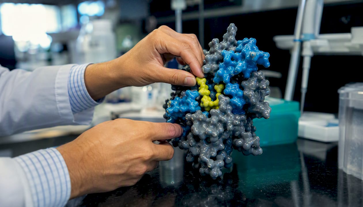
The lock-and-key model treats both protein and ligand as rigid. Induced fit allows the protein to rearrange upon ligand binding. Conformational selection proposes that the protein pre-samples multiple conformations in solution and the ligand stabilizes one of them. Real binding events mix all three mechanisms, often within the same target depending on the ligand chemotype. For docking, this matters because a rigid-receptor run implicitly assumes lock-and-key, which fails for targets with known induced pockets.
What does a standard docking workflow look like?
Step-by-step from structure to hit list
A clean workflow prevents the most common failure modes before the docking run even starts. Structure and ligand preprocessing is often the most time-consuming phase of a docking project, and small errors at this stage, a missing loop, a wrong protonation state, a box that clips the binding site, can invalidate every downstream result.
-
Target selection and structure curation. Download the PDB entry or retrieve an AlphaFold model when no experimental structure exists. Remove crystallographic waters selectively (keep those that mediate key contacts), strip non-relevant ligands and buffer molecules, model missing loops with tools such as Modeller or Prime, and assign protonation states at the target pH using Propka, H++ or the Protein Preparation Wizard in Schrödinger Suite.
-
Binding-site definition. Use the co-crystallized ligand centroid when available. For apo structures, run cavity-detection tools such as SiteMap, fpocket, or DoGSiteScorer. Define the docking box with at least 10 Å padding around the known or predicted site; for blind docking, cover the full protein surface.
-
Ligand library curation. Enumerate tautomers and protonation states at physiological pH (LigPrep, RDKit, OpenBabel). Assign stereochemistry explicitly; never dock a racemic mixture as a single structure. Generate 3D conformers with OMEGA, RDKit ETKDG, or Corina. Filter by Lipinski Ro5 or target-specific physicochemical rules before docking to reduce library size.
-
Docking run setup. Choose the sampling algorithm and scoring function appropriate to throughput needs (see the software section). Set the number of poses per ligand to retain (typically 5–20 for VS, up to 50 for lead optimization). Enable flexible side chains for key residues if the tool supports it.
-
Post-docking filters. Apply interaction fingerprint filters (must-have H-bond to catalytic residue), strain energy cutoffs, and PAINS/aggregator filters. Cluster poses by RMSD to remove redundant solutions.
-
Visual inspection and prioritization. Examine top-ranked poses in PyMOL, UCSF Chimera, or Maestro. Confirm the ligand fits the pocket without clashes, forms expected interactions, and matches SAR if known compounds are available as controls.
Decision rules worth keeping in mind:
- Use a single, well-resolved crystal structure for targets with minimal known flexibility.
- Switch to ensemble docking when multiple experimental conformers exist or MD reveals pocket breathing.
- Size the docking box to the binding site, not the whole protein, except for blind docking experiments.
- Keep 5–10 known actives and decoys in every run as internal controls to catch setup errors early.
Pro Tip: Before running a full library, always re-dock the co-crystallized ligand and verify the top pose reproduces the experimental binding mode within 2 Å RMSD. If it does not, fix the setup before spending compute on the full screen.
How do search algorithms handle receptor and ligand flexibility?
Docking is fundamentally a sampling problem: the algorithm must explore the rotational, translational, and conformational space of the ligand (and, to varying degrees, the receptor) to find the lowest-energy pose. Protein flexibility is the primary bottleneck for pose prediction accuracy; most tools still assume a fixed backbone, which works well for rigid, well-defined pockets but fails for targets with induced conformational changes.

Major algorithm families
Systematic/grid-based search exhaustively samples discrete rotational and translational increments. Thorough but computationally expensive; practical only for small ligands or narrow binding sites.
Stochastic genetic algorithms (used in AutoDock and GOLD) encode the ligand pose as a chromosome and evolve populations of solutions toward lower energy. Fast convergence, good for flexible ligands, but sensitive to population size and termination criteria.
Monte Carlo methods make random perturbations to pose and accept or reject them by a Boltzmann criterion. Glide's GlideScore uses a Monte Carlo-like minimization in its SP and XP modes. Good for local refinement; less efficient for global search.
Fragment-based incremental construction (DOCK, Surflex-Dock) builds the ligand incrementally from a rigid core, adding flexible fragments one at a time. Efficient for large, flexible molecules.
MD-based and enhanced sampling methods (metadynamics, replica exchange, steered MD) provide the most physically realistic sampling but are orders of magnitude slower. Reserved for final pose refinement or when the binding mechanism itself is under study.
Strategies for receptor flexibility
| Strategy | What it does | When to use it |
|---|---|---|
| Rigid receptor | Fixed backbone and side chains | Well-resolved crystal structure, rigid pocket |
| Flexible side chains | Rotamer sampling for key residues | Known side-chain rearrangements at the binding site |
| Soft docking | Reduced van der Waals radii to tolerate minor clashes | Moderate induced fit, fast screening |
| Ensemble docking | Multiple receptor conformations from MD or experimental structures | Known conformational heterogeneity, cryptic pockets |
| Induced-fit docking (IFD) | Full side-chain and backbone relaxation around the docked pose | Lead optimization, large structural rearrangements |
Ensemble docking using multiple receptor conformations from MD or experimental structures is a practical strategy for protein flexibility, but using too many conformers increases false positives and compute cost. A practical rule: generate 5–10 representative conformers from a clustering of an MD trajectory rather than docking against every frame.
When a target has a known induced pocket change (e.g., DFG-in vs. DFG-out in kinases, or an allosteric site that opens only in the active state), generate conformers from experimental structures in both states or run a short unbiased MD simulation (50–100 ns) and cluster the trajectory before docking.
What scoring functions actually measure, and when they fail
Scoring functions are the heart of docking and its most persistent weakness. They approximate ΔG quickly enough to rank millions of poses but sacrifice accuracy to do it. Molecular docking's predictive power depends critically on the scoring function used, and no single function dominates across all target classes.
Four scoring function families
Physics-based (force-field) scoring computes electrostatic and van der Waals terms from molecular mechanics force fields (AMBER, CHARMM, OPLS). Interpretable and transferable, but ignores solvation entropy and is slow when computed rigorously. AutoDock's original scoring function is a hybrid of this type.
Empirical scoring functions fit a weighted sum of interaction terms (H-bonds, hydrophobic contacts, rotatable bonds) to experimental binding data. Fast and well-calibrated for drug-like molecules near the training set. GlideScore (Glide) and ChemScore (GOLD) are prominent examples. They fail when the target or chemotype diverges from the training data.
Knowledge-based (statistical potential) scoring derives pairwise atom-atom potentials from the statistical distribution of contacts in PDB structures. AutoDock Vina's scoring function is a hybrid empirical/knowledge-based approach. Broad applicability, but dependent on PDB coverage of the target class.
Machine-learning scoring functions train neural networks or gradient-boosted models on large docked-pose datasets. They capture nonlinear interaction patterns that classical functions miss. The transition to ML-based scoring is the active frontier in the field, but these models need large, high-quality training sets and can overfit to PDB biases. Scoring functions are grouped into physics-based, empirical, and knowledge-based families; accurate free-energy methods like FEP/TI are more rigorous but computationally expensive.
Scoring trade-offs at a glance
| Scoring type | Speed | Accuracy (pose) | Accuracy (affinity) | Interpretability | Data requirements |
|---|---|---|---|---|---|
| Physics-based | Moderate | Good | Moderate | High | Low |
| Empirical | Fast | Good | Moderate | Moderate | Medium |
| Knowledge-based | Fast | Moderate | Moderate | Low | Medium |
| ML-based | Fast (inference) | Variable | Variable–High | Low | High |
| MM-GBSA rescoring | Slow | High | Good | Moderate | Low |
| FEP/TI | Very slow | Very high | High | Moderate | Low |
When to rescore and how
Raw docking scores are sufficient for initial VS ranking. For lead candidates, MM-GBSA rescoring on short MD snapshots improves affinity ranking at moderate compute cost. Reserve FEP or thermodynamic integration (TI) for the final 10–20 compounds in a lead optimization series, where 0.5 kcal/mol accuracy matters.
How should you validate a docking protocol?
Validation is not optional. A docking protocol that has not been benchmarked against known data is a hypothesis generator at best and a source of expensive false leads at worst. Benchmarking should separate pose prediction from enrichment performance and use community datasets like DUD-E and LIT-PCBA for standardized retrospective tests.

Metrics that matter
RMSD (root-mean-square deviation): measures pose prediction accuracy by comparing the docked pose to the experimental binding mode. A pose within 2 Å RMSD of the crystal structure is conventionally considered correct. RMSD alone does not tell you whether the protocol enriches actives over decoys.
Enrichment factor (EF): the ratio of actives recovered in the top X% of the ranked list versus random selection.
ROC/AUC: the area under the receiver operating characteristic curve measures overall discrimination between actives and decoys across all thresholds. AUC of 0.5 is random; above 0.7 is generally considered useful for VS.
BEDROC (Boltzmann-Enhanced Discrimination of ROC): a weighted variant of AUC that emphasizes early enrichment. More sensitive than AUC for VS applications where only the top-ranked compounds get tested.
Community benchmark datasets
DUD-E (Directory of Useful Decoys, Enhanced): 102 targets with experimentally confirmed actives and property-matched decoys. The standard for retrospective VS benchmarking. Known limitation: decoys are topologically dissimilar to actives, which can inflate apparent enrichment.
LIT-PCBA: a more recent dataset derived from PubChem confirmatory assays, with more realistic active/decoy ratios and less artificial separation. Harder than DUD-E and considered a more stringent test of VS performance.
Retrospective vs. prospective validation
Retrospective validation re-ranks known actives and decoys using the protocol you plan to deploy. It confirms the protocol can recover known binders but does not guarantee it will find new ones. Prospective validation tests predictions experimentally, the only true measure of a protocol's real-world utility. Every published docking study should include at minimum a retrospective benchmark; prospective validation with SPR, ITC, or a biochemical assay is the gold standard for confirming the protocol works on your specific target.
Validation checklist for methods sections:
- Report software name and version, scoring function, and all non-default parameters.
- State the benchmark dataset used and the metric(s) reported (RMSD, EF₁%, AUC, BEDROC).
- Include at least five known actives and a matched decoy set as internal controls.
- Report random seed(s) for reproducibility.
- Describe how poses were selected for experimental follow-up (score cutoff, visual inspection criteria).
Which docking tool should you use for your research task?
The right tool depends on throughput requirements, the degree of protein flexibility, and whether the project is in the VS or lead optimization phase. Below is a practical comparison of the tools researchers reach for most often.
Practical selection guidance
For large-scale virtual screening (>100K compounds): AutoDock Vina and FRED offer the best throughput at low or no cost. Vina's open-source nature makes it easy to parallelize on HPC clusters. FRED's shape-based scoring is fast and less sensitive to minor protonation errors.
For lead optimization and pose quality: GOLD and Glide XP consistently rank among the most accurate for pose prediction on drug-like targets. Glide's induced-fit docking (IFD) protocol handles large conformational changes better than most alternatives. GOLD's multiple scoring functions (GoldScore, ChemScore, ASP) support consensus scoring natively.
For academic projects with limited budget: AutoDock and AutoDock Vina remain the most widely used tools in published literature, with extensive community documentation and free access. DOCK is a strong alternative for fragment-based approaches.
On AlphaFold as a structural input: AlphaFold-predicted structures are now widely used as docking inputs when experimental coordinates are unavailable, but local model uncertainty around loops and binding-site residues requires careful inspection before docking. Check the per-residue confidence score (pLDDT); residues below 70 in the binding site warrant caution. Pair AlphaFold models with computational protein modeling advances to validate and refine predicted binding pockets before committing to a full screen.
When should you move beyond raw docking scores?
Raw docking scores are fast approximations. For the top candidates from a VS campaign, higher-confidence refinement methods improve the reliability of affinity ranking before committing to synthesis or assay.
MM-GBSA and MM-PBSA rescoring
Molecular mechanics combined with generalized Born or Poisson-Boltzmann surface area (MM-GBSA/MM-PBSA) rescoring re-evaluates top poses with an implicit solvent model after short MD relaxation. It captures conformational strain and solvation effects that docking scoring functions miss. Correlation with experimental IC₅₀ values improves substantially over raw docking scores for congeneric series.
Setup pitfalls that invalidate MM-GBSA runs:
- Insufficient MD sampling (less than 5 ns for flexible loops near the binding site).
- Wrong protonation states carried forward from docking without re-checking at the MD force field level.
- Missing structural waters that mediate key contacts (these must be retained explicitly).
- Ignoring counterions in charged binding sites.
FEP and thermodynamic integration
Free energy perturbation (FEP) and thermodynamic integration (TI) are the most rigorous methods for predicting relative binding free energies. They require exhaustive conformational sampling with explicit solvent and are computationally expensive, typically 10–100 GPU-hours per compound pair. Accurate binding free energy prediction requires exhaustive sampling and explicit solvent methods such as FEP or TI, appropriate for final lead optimization rather than large-scale screening.
The recommended escalation ladder:
- Docking score: rank the full library.
- Consensus scoring or ML rescoring: filter top 1–5%.
- MM-GBSA: rank the top 100–500 poses.
- Short MD + MM-GBSA: validate top 20–50 compounds.
- FEP/TI: final ranking of 5–20 lead candidates before synthesis.
What are the most common docking pitfalls, and how do you avoid them?
Most docking failures trace back to a handful of recurring mistakes. Catching them before the run saves weeks of wasted compute and false experimental leads.
High-probability failure modes
- Missing loops or residues near the binding site. A gap in the backbone changes the pocket shape and volume. Model missing residues with Modeller, Rosetta loop modeling, or Prime before docking.
- Wrong protonation states. Histidine tautomers, aspartate/glutamate protonation, and cysteine ionization state all shift at different pH values. Use Propka or H++ to predict states at your target pH, and consider running docking at two or three protonation states for ambiguous residues.
- Ignored structural waters. Conserved waters in the binding site (e.g., the catalytic water in serine proteases, bridging waters in kinase hinge regions) mediate key interactions. Stripping all waters before docking removes these contacts and produces incorrect poses.
- Metal coordination geometry. Zinc, magnesium, and iron centers require specialized parameterization. Standard force fields misrepresent metal-ligand bonds; use metal-aware scoring (GOLD's ASP function handles zinc well) or apply geometric constraints.
- Overreliance on raw docking scores. Score distributions often overlap between actives and inactives. A compound ranked first by docking score is not necessarily the best binder; always combine score with visual inspection and interaction fingerprint analysis.
- Ignoring tautomers. A ligand that exists as multiple tautomers in solution may bind in a tautomeric form different from the most stable one. Enumerate tautomers explicitly during ligand preparation.
Mitigations at a glance
- Run the re-docking self-test (co-crystallized ligand, RMSD < 2 Å) before every new target.
- Keep 5 known actives and 50 decoys in every VS run as internal controls.
- Use structural visualization techniques to inspect every top-ranked pose manually before advancing to assay.
- For metalloproteins, use GOLD with ASP scoring or apply distance/angle constraints to the metal center.
- Validate hits orthogonally: SPR or ITC for binding confirmation, thermal shift for target engagement, and a functional assay for activity.
Pro Tip: Binding kinetics (on/off rates, residence time) can matter more than equilibrium Kd for in vivo efficacy. If your target has a known residence time requirement, plan SPR experiments alongside docking to measure koff, not just affinity. Residence time may be more relevant to biological effect than raw Kd in many drug discovery scenarios.
What can docking realistically deliver in drug discovery?
Docking is a hypothesis-generation tool, not a prediction engine. Understanding what it reliably delivers, and where it falls short, prevents misaligned expectations and wasted resources.
Use cases and expected outcomes
| Application | What docking delivers | Realistic hit rate | Recommended follow-up |
|---|---|---|---|
| Large-scale VS (>100K cpds) | Prioritized hit list, with an expected small fraction of actives | 1–10% of top-ranked compounds confirm in assay | Biochemical assay, SPR/ITC for top 50–100 |
| SAR rationalization | Pose-based explanation of potency differences | Qualitative; confirms SAR trends | Mutagenesis, X-ray of key analogs |
| Mechanistic hypothesis | Proposed binding mode for mutagenesis design | Directional; not quantitative | Mutagenesis, cryo-EM, NMR |
| Hit-to-lead optimization | Ranked analogs for synthesis prioritization | A moderate rank correlation with IC₅₀ in congeneric series | MM-GBSA, FEP for final 10–20 leads |
| Covalent inhibitor design | Warhead placement and covalent bond geometry | Qualitative pose; no covalent ΔG | Covalent docking (CovDock, AutoDock), mass spec confirmation |
Special cases worth flagging
Membrane proteins (GPCRs, ion channels, transporters): docking against membrane proteins requires the receptor in a lipid bilayer context or at minimum a membrane-mimetic environment. Binding pockets in GPCRs are well-defined in active and inactive state structures, but the orthosteric and allosteric sites behave differently. Use state-specific structures and validate with functional assays.
Metalloproteins: as noted above, standard scoring functions underperform. GOLD's ASP function or specialized metal-aware force fields (MCPB.py for AMBER parameterization) are the practical choices.
Covalent inhibitors: standard docking does not model covalent bond formation. Use CovDock (Schrödinger) or AutoDock's covalent docking mode, which places the warhead at the reactive residue and docks the rest of the molecule. Confirm covalent engagement by mass spectrometry.
Integrative approaches: combining docking with cryo-EM, NMR restraints, or mutagenesis constraints improves hit rates by constraining the search space. When sparse experimental data is available (a few NOE distances, a cryo-EM density map at 4–6 Å resolution), incorporating those restraints into the docking run dramatically reduces false positives. Understanding why protein structure accuracy matters for docking outcomes is especially relevant here: the quality of the receptor model sets the ceiling on what any docking protocol can achieve.
A reproducible docking checklist for methods sections and SOPs
The checklist below is written to be copied directly into a methods section or SOP. Every item maps to a decision that affects reproducibility and result quality.
Pre-docking preparation
- Retrieve and inspect the receptor structure. Download from RCSB PDB or AlphaFold EBI server. Record PDB ID, resolution, and experimental method. Check for missing residues (SEQRES vs. ATOM records), alternate conformations, and crystal contacts near the binding site.
- Model missing residues. Use Modeller 10.x, Prime (Schrödinger), or Rosetta loop modeling. Verify the modeled loop does not occlude the binding site.
- Assign protonation states. Run Propka 3.x or H++ at pH 7.4 (or target-relevant pH). Manually check histidine tautomers and cysteines. Document all non-default assignments.
- Retain or remove waters. Keep crystallographic waters within 5 Å of the binding site that form bridging contacts. Remove bulk solvent.
- Define the binding box. Center on the co-crystallized ligand or predicted cavity centroid. Set box dimensions to at least 10 Å beyond the ligand extent. Record box center coordinates and dimensions.
- Prepare the ligand library. Enumerate tautomers (Epik, RDKit, OpenBabel). Assign protonation states at pH 7.4. Enumerate stereocenters explicitly. Generate 3D conformers (OMEGA, RDKit ETKDG). Filter by MW ≤ 500, cLogP ≤ 5, and PAINS/aggregator flags.
Docking run
- Select the docking tool and mode. Document software version and all non-default parameters (number of GA runs, population size, exhaustiveness, grid spacing).
- Run the self-docking validation. Re-dock the co-crystallized ligand. Confirm RMSD < 2 Å for the top-ranked pose. If RMSD > 2 Å, diagnose before proceeding.
- Run the full docking campaign. Retain 5–20 poses per ligand. Record all scores and pose coordinates.
Post-docking
- Apply interaction filters. Require key pharmacophoric interactions (e.g., H-bond to hinge residue in kinases). Remove poses with clashes (internal strain energy > 10 kcal/mol).
- Rescore top candidates. Apply consensus scoring or MM-GBSA for the top 1–5% of ranked compounds.
- Visual inspection. Examine top 50–100 poses in PyMOL or UCSF ChimeraX. Flag compounds with unrealistic geometries.
- Report metrics. Include EF₁%, AUC, and BEDROC for the benchmark set. State the random seed(s) used.
Reporting standards
Include in the methods section: software name and version, scoring function, box definition, protonation tool and pH, ligand preparation pipeline, number of poses retained, post-docking filters applied, benchmark dataset and metrics, and random seed(s). Include in supplementary: full ranked hit list with scores, RMSD values for the self-docking test, and the benchmark ROC curve.
When to outsource
Consider engaging a dedicated computational service when: the library exceeds 500K compounds and local HPC resources are insufficient; the target requires ensemble generation from long MD simulations; the project needs a reproducible, documented pipeline for regulatory submission; or the team lacks expertise in a specific step (metal parameterization, covalent docking, FEP setup). Practical guidance on when docking projects benefit from outsourcing covers how to scope a vendor engagement and what deliverables to request.
Pro Tip: When writing the methods section for publication, include the docking box coordinates and the random seed. These two items, almost always omitted, are what prevent other labs from reproducing your screen exactly.
A perspective on what docking projects actually look like in practice
The gap between a textbook docking workflow and a real project is wider than most papers suggest. The preprocessing phase, assigning protonation states, modeling loops, deciding which waters to keep, routinely takes longer than the docking run itself. A 48-hour GPU job is easy to set up; getting the receptor right takes days of careful QC.
The second underappreciated reality is that scoring function choice matters less than structure quality. Two groups running the same library against the same target with different tools (say, AutoDock Vina versus Glide SP) will often produce correlated hit lists if both started from a well-prepared receptor. Run the same tools against a poorly prepared structure and the results diverge badly. The receptor is the experiment.
ML-based scoring functions are genuinely exciting, but the field has not yet converged on a standard. Models trained on PDB-derived data inherit PDB biases: overrepresentation of certain target families, co-crystallization artifacts, and the fact that most deposited structures are of high-affinity binders. A model that performs brilliantly on DUD-E may fail on a novel target class with sparse structural data. The honest position is that ML rescoring is a useful addition to the pipeline for well-represented target families, not a replacement for physical reasoning.
One operational observation worth stating plainly: the projects that produce the most reliable hit lists are the ones where the computational team and the experimental team talk to each other before the screen runs, not after. Knowing which assay will be used, what the throughput limit is, and what a "hit" means in that assay changes every decision from box size to the number of poses to retain.
Innovabiotech supports your docking projects from setup to validated hits
Running a rigorous docking campaign, one with proper preprocessing, ensemble generation, MM-GBSA rescoring, and a documented benchmark, requires both computational infrastructure and the scientific judgment to make the right calls at each step. Innovabiotech delivers exactly that for biotech and pharma teams who need results they can trust and reproduce.
Innovabiotech's computational biology team in San Francisco handles the full pipeline: structure curation and protonation, large-scale virtual screening with AutoDock Vina, Glide, or GOLD depending on project requirements, ensemble generation from MD, MM-GBSA rescoring, and FEP setup for lead optimization. Projects are scoped per engagement with full documentation suitable for publication or regulatory use. Whether you need a one-time VS campaign against a novel target or an ongoing protein design and docking service integrated with your experimental assay team, Innovabiotech can scope and deliver it. For docking-informed peptide affinity optimization, the team applies structure-based design alongside binding affinity prediction to accelerate hit-to-lead cycles. Contact Innovabiotech to discuss your target, timeline, and deliverables.
Sources
The references below cover the canonical literature, community datasets, and tool documentation researchers need to go deeper on any section of this guide.
- Protein–Ligand Docking in the Machine-Learning Era
- Principles of molecular recognition | Foundations of protein structure
- Insights into Protein–Ligand Interactions: Mechanisms, Models, and Methods
- The Art and Science of Molecular Docking | Annual Reviews
- Alphafold
FAQ
What is protein–ligand docking used for in drug discovery?
Protein–ligand docking is used to predict how a small molecule binds to a target protein and to rank large compound libraries by predicted affinity, enabling virtual screening, SAR rationalization, and hit-to-lead prioritization before experimental assays run.
How accurate are docking scores at predicting binding affinity?
Docking scores correlate with experimental affinity within congeneric series but are unreliable for absolute affinity prediction across diverse chemotypes. MM-GBSA rescoring improves ranking accuracy for top hits; FEP/TI is required for sub-kcal/mol precision in lead optimization.
What RMSD threshold defines a correct docking pose?
A docked pose within 2 Å RMSD of the experimental binding mode (from X-ray crystallography or NMR) is the conventional threshold for a correct pose prediction in the docking literature.
Can you use AlphaFold structures for docking?
Yes, AlphaFold-predicted structures are widely used as docking inputs when no experimental structure is available, but binding-site residues with pLDDT scores below 70 should be treated with caution and ideally refined before running a full screen.
When should a docking project be outsourced to a specialist service?
Consider outsourcing when the library exceeds 500K compounds, the target requires long MD-based ensemble generation, the pipeline needs regulatory-grade documentation, or the team lacks expertise in specific steps such as metal parameterization or covalent docking setup. Innovabiotech scopes and delivers these projects end-to-end.